
Introduction
Designing underfloor heating requires routing a continuous loop of pipe from a heat distributor through every room. Traditionally, engineers hand-sketch paths or use semi‑manual CAD tools—an error‑prone, time‑consuming process.
OptiPipe is a proof‑of‑concept Python library that fully automates this: it models your floor plan, discretizes it into a graph, and uses tree‑search heuristics to lay out pipe loops that
- Maximize floor coverage,
- Adhere to inlets/outlets,
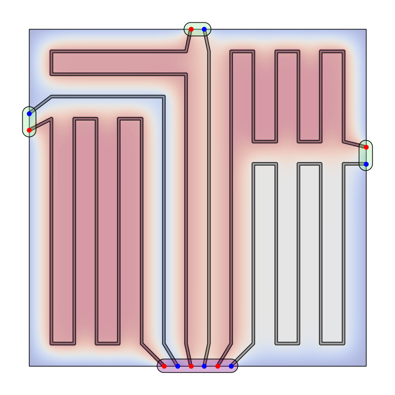
- Visually render the heat diffusion profile.
In this post, we’ll walk through how OptiPipe works, share example results, and show you how to get started.
Why Automate Pipe Routing?
Reduce Manual Labor
Hand‑routing piping for every room—especially irregular layouts—can take hours.Optimize Performance
By exploring many routing possibilities, heuristic search can find layouts that deliver more uniform heat with fewer pressure losses.Visual Feedback
Instant heat‑map visualizations let you see “cold spots” before installation.
Core Concepts
1. Floor Modeling
- Floor: Defines the polygonal boundary of your space.
- Distributor: One or more inlet/outlet node pairs where the manifold sits.
- RoomConnection: Pairs of input/output nodes representing each room segment with associated heat‑loss factors.
2. Graph Discretization
OptiPipe takes your continuous floor polygon and overlays a uniform grid (configurable cell size). Each grid cell becomes a graph node; adjacent cells connect with weighted edges that penalize sharp turns and overlap with walls.
3. Routing Strategies
Naive Router
Uses Dijkstra’s shortest‑path algorithm between each distributor node and room node along centerlines. Fast, produces visually clean loops, but may leave uncovered regions.Heuristic Router
Builds on the naive path: it recursively explores unused grid areas (a DFS with backtracking), scores each candidate path by added coverage and total length, and respects a time budget to return the best solution found.
4. Heat‑Distribution Simulation
Once pipes are laid, a convolution‑based solver (GPU accelerated if you have PyTorch+CUD A) diffuses heat from the pipe lines across the floor. You instantly see where temperatures peak or dip.
Quick‑Start Example
Peek under the hood in the Jupyter proof‑of‑concept notebook.
from opti_pipe import Model, Floor, Distributor, Node, NodeType, RoomConnection
from opti_pipe.utils import load_config
from opti_pipe.router import HeuristicRouter

# Load YAML‑based defaults
config = load_config("data/config.yaml")

# Define a simple 5×5 m room
floor = Floor(config, corners=[(0,0), (0,5), (5,5), (5,0)])

# Manifold inlet/outlet at bottom wall
distributor = Distributor(
    config,
    nodes=(
        Node(config, 2.0, 0, node_type=NodeType.INPUT),
        Node(config, 2.2, 0, node_type=NodeType.OUTPUT),
    ),
    heat_per_node=1.0
)

# Single room‑connection opposite the distributor
room_conn = RoomConnection(
    config,
    output=Node(config, 0, 3.75, node_type=NodeType.OUTPUT),
    input=Node(config, 0, 3.5, node_type=NodeType.INPUT),
    heat_loss=0.8
)

# Assemble model, discretize, and route
model = Model(config, target_heat_input=100, floor=floor,
              distributor=distributor, room_connections=(room_conn,))
model.add_graph(grid_size=0.2)

router = HeuristicRouter(config, model, grid_size=0.2)
routed = router.route()

# Render piping + heat‑map
routed.render(show_graph=False, render_heat_distribution=True)
Example Output
Configuration & Extension
All parameters live in data/config.yaml—from pipe thickness and colors to DFS search weights and heat solver settings.
You can:
- Tweak grid resolution (
grid_size) for finer control vs. speed - Swap in your own weight functions in
router/for custom heuristics - Extend the
Modelto support non‑rectangular or multi‑room floor plans
Get Started
Clone & install:
git clone https://github.com/felixscode/opti-pipe.git
cd opti-pipe
pip install -e .
Explore the notebook:
jupyter lab jupyter/proof.ipynbShare feedback or code contributions on the GitHub repo.
Happy piping! — Felix Schelling Spring 2025